Evaluation Isn't One Number: Lessons from a Microservice Fault Classifier
How I built and evaluated FaultTrack, a random forest that classifies microservice faults, and why it scored 0.80 on known systems but 0.57 on unseen systems.
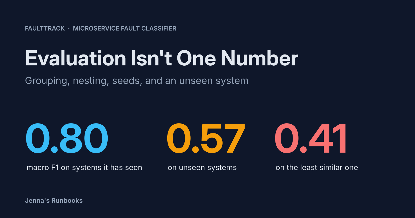
FaultTrack is a classifier that guesses the fault type behind a microservice alert from the surrounding metrics. I used nested, grouped k-fold cross-validation to tune and compare four models. A random forest won, scoring 0.80 macro F1 (a 0-to-1 score averaged across the six fault types) on systems it was trained on, and 0.57 on average on systems it had never seen. A team running it on their own cluster is in the 0.57 case, where more wrong guesses mean misrouted triage and less trust in the tool. The biggest lesson was that evaluation isn’t one number. Grouping, nesting, seeds, and an unseen system changed what my score meant.
The task and the data
FaultTrack looks at the per-service metrics around an alert and answers two questions: which kind of fault is it (CPU, memory, disk, socket, network delay or packet loss), and which service did it most likely start in.
- Data: RCAEval RE2 (Pham et al., WWW 2025 Companion, CC BY 4.0). RE2 has three microservice systems: Online Boutique (OB), Sock Shop (SS) and Train Ticket (TT). Each has 6 fault types injected into 5 services, 3 times each, which gives 90 cases per system, 270 in total.
- Case: One fault injected into one service of one system, for example
re2ob/productcatalogservice_cpu/1. - Rows: An alert doesn't fire at the instant of the fault, so each case gives 5 rows, at detection delays of 0, 30, 60, 90 and 120 s after the injection.
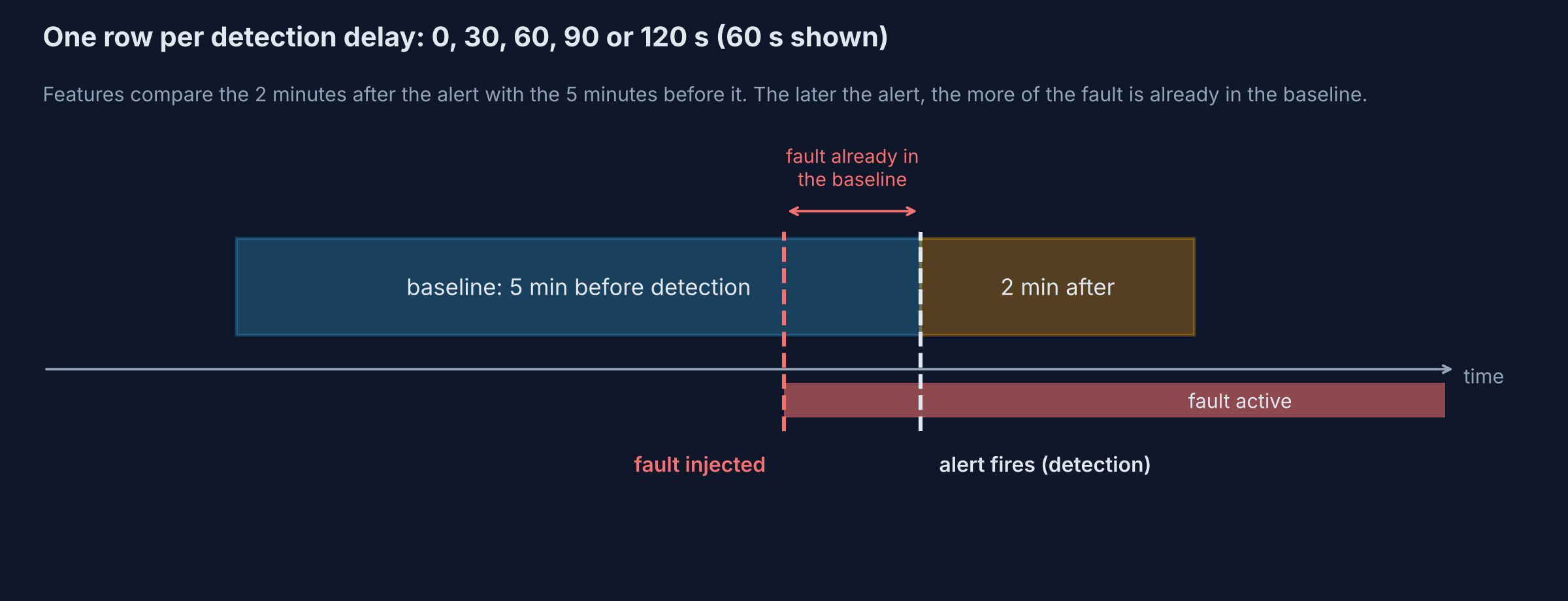
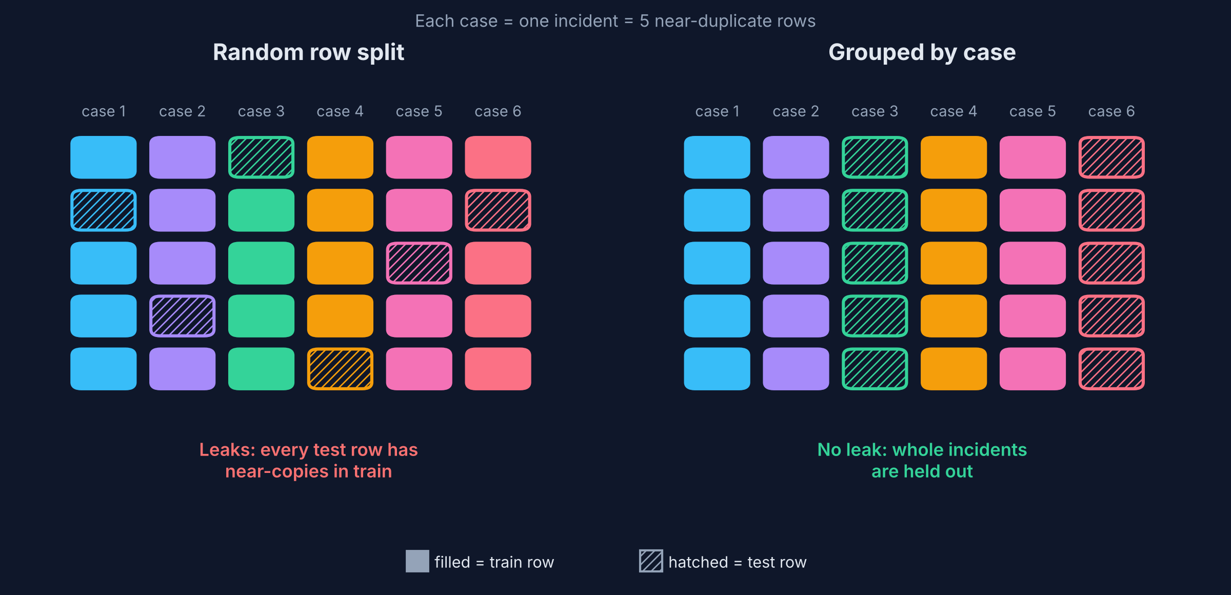
That gives 1,350 rows, and since the 5 rows of a case are near-duplicates, a random split would put rows from the same incident in both train and test. The model would be tested on near-copies of rows it trained on, and score higher than it would on new incidents. That's data leakage, and to prevent this, cross-validation is grouped by case.
How the 0.80 was measured
The headline score comes from a grouped 5-fold cross-validation across all 3 systems, GroupKFold grouped by case, forcing a case's 5 rows to always land on the same side, as in the split diagram above. Macro F1 is measured per fault type, then averaged, so all 6 fault types count equally. The final model scores a macro F1 of 0.799 (the 0.80 above), with individual folds from 0.775 to 0.850.
Grouping isn't enough on its own; scoring a model with the same folds that picked its hyperparameters makes it appear better than it is. Tuning follows a similar approach. The hyperparameter search runs only on the training cases of each of the five folds, and its own split is grouped too. This is nested cross-validation, so the test cases never influence the settings. I compared four models, from simplest to most complex: logistic regression, a decision tree, a random forest and XGBoost. I set the rule in advance: the highest nested mean macro F1 score wins, unless a simpler model is within one fold’s standard deviation of it. The random forest scored highest, with XGBoost within one fold’s standard deviation. The forest is also the simpler of the two, so the tie-break agreed. The shipped model’s settings came from one more search over all the data, on the same folds that produce the 0.799, which could make that score slightly optimistic. Nested CV is the check: it scores the forest at 0.800, and the two agree to within 0.001.
Re-running the final model with fold seeds 0–4 gives means from 0.787 to 0.823, meaning the second decimal is uncertain and differences under about 0.03 aren't real. The model's macro F1 stays between 0.787 and 0.806 at every detection delay, so it doesn't depend on catching the fault the moment it's injected.
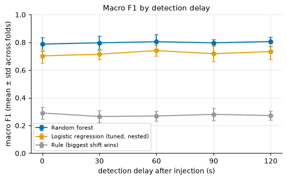
The 0.80 holds up on systems it was trained on, but what about a system it hasn't seen?
The unseen system
Grouped CV mixes cases from all three systems in every fold, so the model is always tested on a system it has already seen other cases of. A team using FaultTrack on its own cluster is running it on a system it has never seen. Leave-one-system-out (LOSO) provides the estimate for that scenario by training on two systems and testing on the third. The three held-out scores averaged 0.57, against 0.80 when the system has been seen. TT is the easiest system when it’s in the training data (0.90), and the hardest when it isn’t (0.41).
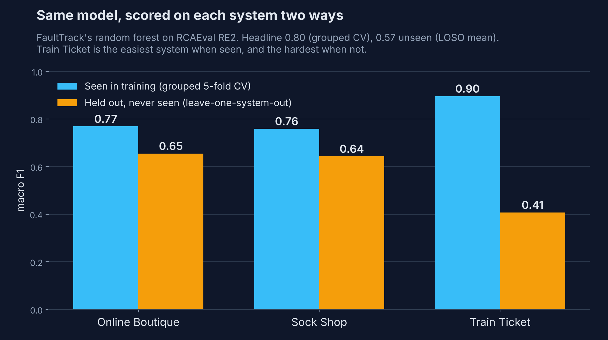
TT differs the most from the other systems in two ways:
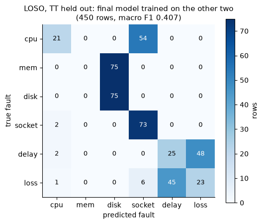
- Size: TT has 68 services against 11 in OB and SS, which sends 54 of 75 CPU rows to socket.
- Telemetry: on TT a memory fault also moves disk I/O, which the other two systems barely show, so the model reads all 75 memory rows as disk faults.
Both appear in TT’s confusion matrix:
Closing the gap, partly
I tried two ways to close the gap:
- Norm-counts: per-service means and fractions instead of sums and counts.
- Relative: each feature standardized within its own system.
TT held out, final model, out of 75 rows per fault.
| Features | cpu → socket | socket → cpu | mem → disk | delay → loss | loss → delay | Macro F1 |
|---|---|---|---|---|---|---|
| Headline | 54 | 2 | 75 | 48 | 45 | 0.407 |
| Norm-counts | 11 | 18 | 74 | 29 | 66 | 0.465 |
| Relative | 14 | 35 | 75 | 58 | 35 | 0.414 |
Norm-counts fixes most of TT's cpu → socket errors, dropping them from 54 to 11, but socket → cpu now rises from 2 to 18, so the two are still confused, just in both directions. Norm-counts raises TT from 0.407 to 0.465, and the LOSO mean across all three systems by 0.024 on average over 5 model seeds. TT's mem → disk errors barely moved under either experiment (74–75 of 75), and relative features hardly helped (TT 0.414). The norm-counts gain was consistent, but below the 0.05 my project rules treat as a real metrics change, and regenerating everything that close to submission wasn’t worth it. LOSO stayed about 0.20 below grouped CV.
Some things do carry over to an unseen system. The final model rarely confuses a resource fault (CPU, memory, disk, socket) with a network fault (delay, loss): only about 2% of rows. The suspect-service rule isn't trained, so it has no seen/unseen gap: its hit rate is 88%, 97% and 85% on OB, SS and TT.
The takeaway, and the fine print
While the 0.80 wasn’t wrong, it wasn't answering the question that would be asked by the people most likely to use it. A team running FaultTrack on their own cluster will be asking how well it classifies faults on a system it wasn’t trained on, and the answer to that is 0.57.
Report how the model does where it will actually run, not only where it was trained.
That's why the README's Results section gives the 0.57 right next to the 0.80, with its own subsection on generalizing to an unseen system.
A few limits:
- Small data: 270 cases, 45 per fault type, across three systems, so the scores move with small changes in the data or the fold split.
- Injected faults, not real incidents: real incidents overlap, are messier, and aren’t balanced across types.
- Five windows per case aren’t independent: the effective sample is closer to 270 than 1,350.
- Probability calibration wasn’t checked: the API returns class probabilities, and a 70% shouldn’t be read as “70% likely” until it’s checked.
Try it yourself
Everything here is in the repo, free to reuse:
| What | Why you might want it |
|---|---|
| Feature table (attribution) | 1,350 rows ready to model, without the 4 GB download. CC BY 4.0, so credit RCAEval. |
Grouped and nested CV (grouped_cv) |
Case-grouped folds with nested tuning in one function when you pass it a search. |
Leave-one-system-out (leave_one_system_out) |
The unseen-system check, a pattern you can adapt to data with a system or site column. |
guard_splits.py hook |
A Claude Code hook that blocks common row-level split calls in agent edits. |
One approach to the unseen-system gap is few-shot adaptation: using 10 labeled examples per fault from the new system, Wang et al. nearly close it for trace-based fault categorization. Have you closed a gap like this on a system your model never saw? Leave a comment. I’d like to hear from you: what worked, the challenges you faced and what you learned.
Sources
FaultTrack
Data
- Pham et al., RCAEval: A Benchmark for Root Cause Analysis of Microservice Systems with Telemetry Data, WWW 2025 Companion. Dataset: Zenodo, CC BY 4.0
References
- Dehghani et al., Subject Cross Validation in Human Activity Recognition, arXiv, 2019
- Cawley & Talbot, On Over-fitting in Model Selection and Subsequent Selection Bias in Performance Evaluation, JMLR, 2010
- Wang et al., Cross-System Categorization of Abnormal Traces in Microservice-Based Systems via Meta-Learning, FSE 2025
- Zhang et al., Failure Diagnosis in Microservice Systems: A Comprehensive Survey and Analysis, arXiv
scikit-learn 1.9 docs
Built with Claude Code. Written by me, with illustrations, editing feedback and fact-checking support from Claude. The design, decisions, and final fact-checking are mine.
About the author
- Hi there! I'm a Cloud Engineer & SRE, documenting my transition into AI/ML Platform Engineering. I write technical deep-dives, hands-on implementation guides, CLI helper scripts, and visual architectures covering cloud, infrastructure, orchestration, governance, and modern AI runtimes.
Comments
Join the discussionNo comments yet. Be the first to comment.
MLOps & Reliability
The automation, observability, security, and cost controls that keep production systems reliable, including the ML and AI systems that run on them. Covers IaC (Terraform), event-driven automation (Lambda, SES), CI/CD (GitHub Actions), FinOps, security and least privilege (including AI agents and MCP), and model evaluation and monitoring.